Align function

Often, one of the first steps in order to analyse a time-series that is dense or has unequally spaced observations is to align it on an equally-spaced time grid where each time-point represents an aggregation between itself and the previous time-point.

Computing and plotting the count of the observations over each interval is useful (among other things) to catch data that are missing over a large period. Besides the count, the mean, median, min and max are often useful too.

For all these tasks we can use ztsdb's versatile align function (for a more in-depth description of this function see the reference section Align operations).

Implementation of a grid alignment function

Here is an implementation in ztsdb of a grid alignment function (this and all the following code below can be found here):

grid_align <<- function(z,                         # time-series
                        by,                        # the grid size
                        method,                    # "count", "min", "max", "median", "mean", "closest"
                        ival=by,                   # the interval size
                        start=head(zts.idx(z),1),  # start of the grid
                        end=tail(zts.idx(z),1),    # end of the grid
                        tz=NULL)                   # time zone when using 'period'
{
  if (typeof(by) == "duration") {
    grid <- seq(start+by, end, by=by)
    if (tail(grid,1) < end) {
      c(--grid, tail(grid,1) + by)
    }
  }
  else if (typeof(by) == "period") {
    if (is.null(tz)) stop("tz must be specified when 'by' is a period")
    grid <- seq(`+`(start,by,tz), end, by=by, tz=tz)
    if (tail(grid,1) < end) {
      c(--grid, `+`(tail(grid,1),by,tz))
    }
  }
  else stop("invalid type for 'by', must be 'duration' or 'period'")

  align(z, grid, -ival, as.duration(0), method=method, tz=tz)
}

A few elements to note about the above code:

• The function essentially does two things. First it constructs a grid with appropriate start/end times and spacing, and then it calls the align function to perform the alignment of the given time-series on this grid.

• The grid construction is different when by has type period from when it has type duration because operations with period need an associated time zone. See the discussion about period here.

• We use the pass by reference operator -- in the expression c(--grid, tail(grid,1) + by) to modify grid in place and thus avoid a copy.

• The align method will, for each time point x of the time-series, include the time point x - ival and exclude the time point x. An ival smaller than by may be specified in order to obtain a sample.

After having defined grid_align, the definition of the density function is then trivial because it is just one particular case:

density <<- function(z, by, ival=by, start=head(zts.idx(z),1), end=tail(zts.idx(z),1), tz=NULL)
  grid_align(z, by, "count", ival, start, end, tz)

Using the density function

First, let's initialize a session either by starting a ztsdb instance that we will use as a client or by starting a normal R session. In the latter, the ztsdb interface package rztsdb as well as the xts time-series package must be loaded (this step is not necessary if these queries are being run from a ztsdb client):

library(rztsdb)
library(xts)

In this newly created local session, let's create a variable to hold the time-zone in which we'll be working (so we don't have to type it out in full every time we will need it) and let's create a connection to a remote ztsdb instance (from here, the code and queries are identical in an R session as well as on the ztsdb command line):

tz <- "America/New_York"
c1 <- connection(ip="127.0.0.1", port=12300)

Now, let's create a time-series to play with on the remote ztsdb instance. This time series has 2e6 entries, with time-points uniformly randomly spaced; it also has a few days gap in the midle and a different density before and after the gap:

c1 ? { start <- as.time("2015-01-01 00:00:00 America/New_York")
       idx <- c(start,
                start + cumsum(runif(1e6-1))*as.duration("00:00:01"),
                start + 10*as.duration("24:00:00") + cumsum(runif(1e6,0,0.5))*as.duration("00:00:01"))
       z   <<- zts(idx, matrix(1:2e6, 2e6, 1)) }

A few elements to note on the above code:

• The result of the expression is not z because the last statement in the expression list is an assignment. Instead, this query returns TRUE.

• The special assign operator <<- was used for the assignment to z. This is not necessary if z is only ever going to be accessed by the session that created it. But if it needs to be accessed by other instances or remain when the connection is torn down, then it must be assigned in the global environment.

• Although z is defined in the global environment, it is not persistent. To make it persistent we would use:

  z <<- zts(idx, matrix(1:2e6, 2e6, 1), file="/dir/to/store/z")
  

We are now ready to try a few density queries for various time intervals:

minutes <- (c1 ? density(z, as.duration("00:01:00")))
hours   <- (c1 ? density(z, as.duration("01:00:00")))
days    <- (c1 ? density(z, as.period("1d"), tz=++tz))
days2   <- (c1 ? { start  <- floor(head(zts.idx(z),1), "day", tz=++tz)
                   density(z, as.period("1d"), start=start, tz=++tz) })

Note that the difference between days and days2 is that the latter query forces the grid to start on a day boundary (this is for illustrative purpose as in this example z starts on a day boundary).

When running these queries from an R session, minutes, hours and days are of type xts. It is then straightforward to use R's plotting capabilities. Here are plots of minutes, hours and days showing the missing data and the uniform density we engineered in our example:

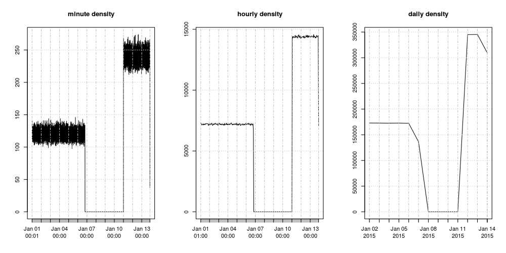
In an R session, the above plot is readily obtained like this:

par(mfrow=c(1,3))
plot.xts(minutes, main="minute density");
plot.xts(hours, main="hourly density");
plot.xts(days, main="dayly density")

For very large time series it can make sense to get the density over a sample rather than over the whole time-series. It is possible to take a minute interval over an hourly grid like this:

hourly_minute_sample <- (c1 ? density(z, as.duration("01:00:00"), ival=as.duration("00:01:00")))

Here is a plot of the hourly minute sample:

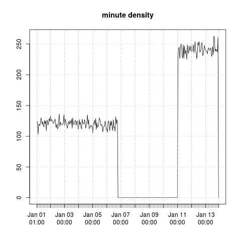
On my slightly older hardware (~2011 Xeon E7-4850 2GHz, 1333MHz DDR3), calculating the minute density over a time-series of one billion observations takes around 14 seconds. Calculating the hourly minute density, i.e. hourly samples, takes a fraction of a second.

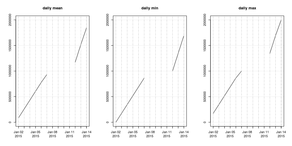
Using the grid_align function

The more general grid_align function can be used in the same way to compute the mean, median, min and max.

days_mean <- (c1 ? grid_align(z, as.duration("24:00:00"), method="mean"))
days_min  <- (c1 ? grid_align(z, as.duration("24:00:00"), method="min"))
days_max  <- (c1 ? grid_align(z, as.duration("24:00:00"), method="max"))

Here is a plot of the dayly mean, min and max:

Conclusion

We have shown part of what can be achieved when using the align function with a grid. align and its cousin align.idx are also extremely useful when trying to match up concurrent time series from different sources.

This example also shows the usefulness of having a full programming language in a database management system and the adequacy for this task of the R programming language. The align function, although extremely versatile, can be a little too low level to be used conveniently, but it is extremely easy to write, like we did above, function wrappers around it to extend its power.

This example also illustrates one of the possible workflows between R and ztsdb. Non-trivial queries can be run from R (even on very large time series when using sampling) and the resulting time-series are immediately available in R for analysis/plotting.